Now we are ready to talk about building linear regression models from data. When we have gotten measurement data in experiments, it is important to construct a linear regression model as a predictive model. The basic structure of the linear regression is defined as follows,
where $A\in\mathbb{R}^{n\times m}$ and $b\in\mathbb{R}^{n}$ are given by the measurement. Therefore, building a linear regression is equal to solve the linear system $Ax=b$. Here we just consider the over determined system $n>m$ since it is often what we have in modern data. We will use the least square estimate to solve the vector $x$.
To explain this linear regression more clearly, let’s say that every rows of equation is based on data from an individual medical history. So the equation $a{i1}x_1+\cdots+a{im}x{m}=b{i}$ means the medical case of the $i-th$ person. Every columns of matrix $A$ represent different kinds of risk factors and the vector $b$ means the risk of heart disease. Therefore, we can give a interpretation about linear regression. Linear regression is a best fit model $x$ for what combination of those factors describe best or predict best the future risk of heart disease. Actually it may be driven by the nonlinear system in real world, here we oversimplify this system by using linear regression to approximate it.
Since we consider the overdetermined system, it is hard to find a vector $x$ that exactly solves this linear model. We want to find the best fit vector $x$ that minimizes the error norm between $Ax$ and $b$. In other words, the best fit vector $x$ gives us the best prediction of $b$ given information in $A$. Here we consider a one-dimensional linear regression model since it can be easily plotted in the following figure and gives a geometric interpretation of linear regression. Of course, the conclusion derived in this way is very simple and can be generalized to much higher-dimensional situations.
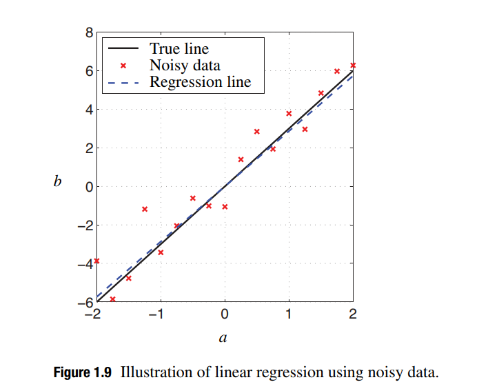
As seen in figure, we will solve the $x$ here that we want is the slope of this fit line. We generalize this interpretation to much higher dimensional case instead of having just one factor that I use to predict $b$. In general, I will find a best fit plane instead of best fit line to approximate the high dimensional data. In one dimensional, $A=\begin{bmatrix} a_1\ a_2\ \cdots\ a_n\end{bmatrix}^{T}$ and $b=\begin{bmatrix}b_1\ b_2\ \cdots\ b_n\end{bmatrix}^{T}$ will be considered. Based on the SVD, we can give the decompostion matrices $U=\frac{A}{\Vert A\Vert_2}$, $\Sigma=\Vert A\Vert_2$ and $V^T=1$ easily. Using Moore-Penrose pseudo inverse of $A$, we can solve the best fit slope $x$ as follows,
Due to the value of the best fit slope, we find that the linear regression can be written as $Ax=AA^{\dagger}b=\frac{AA^T}{\Vert A\Vert_2^2}b$. It means that we project $b$ into the direction of $A$. When we think about the projection, we realize that the normalized matrix $\tilde{A}=\frac{A}{\Vert A\Vert_2}$ satisfies $\tilde{A}^T\tilde{A}=\frac{A^TA}{\Vert A\Vert_2}=1$. From this, we can use this normalized matrix $\tilde{A}$ to derive the projection operator $\tilde{A}(\tilde{A}^T\tilde{A})\tilde{A}^T=\tilde{A}\tilde{A}^{T}=\frac{AA^T}{\Vert A\Vert_2^2}$. This formula can be generalized into higher dimensional case easily.
At last, we consider a very common problem that our data has some outliers in data analysis. As seen in the above figure, these data do not fully mathch our best fitting model. Since the normal data can have some variablity, like Gaussian noisy, our linear regression just is a approximation model to real world. Here we assume that our data has a outlier which is completely different with others. It will bias my distrubution and effect the best fit slope, since the purpose of our derivation is minimizing the sum of the squares of the errors of all of those points to the line. Therefore, it is a big risk we have when we have outliers. Regularly square based on the SVD can handle white noise very well. However, the matrix $A$ will be sensitive to outliers, we will consider in robust statistics.